
Variance
- 2008-03-31 20:23:52
- mlzy
- 原创 11053
Variance,
Beta and Risk 对我来说,是比较容易混淆的概念,需要熟读的~
In
probability theory
and
statistics
, the
variance
of a
random variable
,
probability distribution
, or
sample
is one measure of
statistical dispersion
, averaging the squared distance of its possible values from the
expected value
(mean). Whereas the mean is a way to describe the location of adistribution, the variance is a way to capture its scale or degree ofbeing spread out. The
unit
of variance is the square of the unit of the original variable. The positive
square root
of the variance, called the
standard deviation
, has the same units as the original variable and can be easier to interpret for this reason.The variance of a
real
-valued random variable is its second
central moment
, and it also happens to be its second
cumulant
.Just as some distributions do not have a mean, some do not have avariance as well. The mean exists whenever the variance exists, but notvice versa.
[separator]
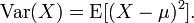
DefinitionIf μ = E(X) is the
expected value
(mean) of the random variable X, then the variance is
 This definition encompasses random variables that are
discrete
,
continuous
,or neither. Of all the points about which squared deviations could havebeen calculated, the mean produces the minimum value for the averagedsum of squared deviations.
This definition encompasses random variables that are
discrete
,
continuous
,or neither. Of all the points about which squared deviations could havebeen calculated, the mean produces the minimum value for the averagedsum of squared deviations.
Many distributions, such as the
Cauchy distribution
,do not have a variance because the relevant integral diverges. Inparticular, if a distribution does not have an expected value, it doesnot have a variance either. The converse is not true: there aredistributions for which the expected value exists, but the variancedoes not.
[
edit
] Discrete caseIf the
random variable
is
discrete
with
probability mass function
p1, ..., pn, this is equivalent to
 (Note: this variance should be divided by the sum of weights in the case of a discrete
weighted variance
.) That is, it is the expected value of the
square of the deviation
of Xfrom its own mean. In plain language, it can be expressed as "Theaverage of the square of the distance of each data point from themean". It is thus the mean squared deviation. The variance of random variable X is typically designated as Var(X),
(Note: this variance should be divided by the sum of weights in the case of a discrete
weighted variance
.) That is, it is the expected value of the
square of the deviation
of Xfrom its own mean. In plain language, it can be expressed as "Theaverage of the square of the distance of each data point from themean". It is thus the mean squared deviation. The variance of random variable X is typically designated as Var(X),
 , or simply σ2.
[
edit
] PropertiesVariance is non-negative because the squares are positive or zero.The variance of a random variable is 0 if and only if the variable isdegenerate, that is, it takes on a constant value with probability 1,and the variance of a variable in a data set is 0 if and only if allentries have the same value.
Variance is
invariant
with respect to changes in a
location parameter
.That is, if a constant is added to all values of the variable, thevariance is unchanged. If all values are scaled by a constant, thevariance is scaled by the square of that constant. These two propertiescan be expressed in the following formula:
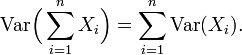
 The variance of a finite
sum
of uncorrelated random variables is equal to the sum of their variances.
The variance of a finite
sum
of uncorrelated random variables is equal to the sum of their variances.
- Suppose that the observations can be partitioned into
subgroupsaccording to some second variable. Then the variance of the total groupis equal to the mean of the variances of the subgroups plus thevariance of the means of the subgroups. This property is known as
variance decomposition or the
law of total variance and plays an important role in the
analysis of variance.For example, suppose that a group consists of a subgroup of men and anequally large subgroup of women. Suppose that the men have a mean bodylength of 180 and that the variance of their lengths is 100. Supposethat the women have a mean length of 160 and that the variance of theirlengths is 50. Then the mean of the variances is (100 + 50) / 2 = 75;the variance of the means is the variance of 180, 160 which is 100.Then, for the total group of men and women combined, the variance ofthe body lengths will be 75 + 100 = 175. Note that this uses N for thedenominator instead of N - 1.In a more general case, if the subgroups have unequal sizes, thenthey must be weighted proportionally to their size in the computationsof the means and variances. The formula is also valid with more thantwo groups, and even if the grouping variable is continuous.
[1]
This formula implies that the variance of the total group cannot besmaller than the mean of the variances of the subgroups. Note, however,that the total variance is not necessarily larger than the variances ofthe subgroups. In the above example, when the subgroups are analyzedseparately, the variance is influenced only by the man-man differencesand the woman-woman differences. If the two groups are combined,however, then the men-women differences enter into the variance also. - Many computational formulas for the variance are based on this equality: The variance is equal to the mean of the squares minus the square of the mean.For example, if we consider the numbers 1, 2, 3, 4 then the mean of thesquares is (1 × 1 + 2 × 2 + 3 × 3 + 4 × 4) / 4 = 7.5. The mean is 2.5,so the square of the mean is 6.25. Therefore the variance is 7.5 − 6.25= 1.25, which is indeed the same result obtained earlier with thedefinition formulas. Many pocket calculators use an algorithm that isbased on this formula and that allows them to compute the variancewhile the data are entered, without storing all values in memory. Thealgorithm is to adjust only three variables when a new data value isentered: The number of data entered so far (n), the sum of the values so far (S), and the sum of the squared values so far (SS). For example, if the data are 1, 2, 3, 4, then after entering the first value, the algorithm would have n = 1, S = 1 and SS = 1. After entering the second value (2), it would have n = 2, S = 3 and SS = 5. When all data are entered, it would have n = 4, S = 10 and SS = 30. Next, the mean is computed as M = S / n, and finally the variance is computed as SS / n − M × M.In this example the outcome would be 30 / 4 - 2.5 × 2.5 = 7.5 − 6.25 =1.25. If the unbiased sample estimate is to be computed, the outcomewill be multiplied by n / (n − 1), which yields 1.667 in this example.
Properties, formal8.a. Variance of the sum of uncorrelated variables
One reason for the use of the variance in preference to othermeasures of dispersion is that the variance of the sum (or thedifference) of uncorrelated random variables is the sum of their variances:
 This statement is often made with the stronger condition that the variables are
independent
, but uncorrelatedness suffices. So if the variables have the same variance σ2, then, since division by n is a linear transformation, this formula immediately implies that the variance of their mean is
This statement is often made with the stronger condition that the variables are
independent
, but uncorrelatedness suffices. So if the variables have the same variance σ2, then, since division by n is a linear transformation, this formula immediately implies that the variance of their mean is That is, the variance of the mean decreases with n. This fact is used in the definition of the
standard error
of the sample mean, which is used in the
central limit theorem
.
That is, the variance of the mean decreases with n. This fact is used in the definition of the
standard error
of the sample mean, which is used in the
central limit theorem
.8.b. Variance of the sum of correlated variables
In general, if the variables are correlated, then the variance of their sum is the sum of their covariances :
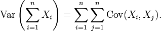 Here Cov is the covariance, which is zero for independent randomvariables (if it exists). The formula states that the variance of a sumis equal to the sum of all elements in the covariance matrix of thecomponents. This formula is used in the theory of
Cronbach's alpha
in
classical test theory
.
Here Cov is the covariance, which is zero for independent randomvariables (if it exists). The formula states that the variance of a sumis equal to the sum of all elements in the covariance matrix of thecomponents. This formula is used in the theory of
Cronbach's alpha
in
classical test theory
.So if the variables have equal variance σ2 and the average correlation of distinct variables is ρ, then the variance of their mean is
 This implies that the variance of the mean increases with theaverage of the correlations. Moreover, if the variables have unitvariance, for example if they are standardized, then this simplifies to
 This formula is used in the
Spearman-Brown prediction formula
of classical test theory. This converges to ρ if ngoes to infinity, provided that the average correlation remainsconstant or converges too. So for the variance of the mean ofstandardized variables with equal correlations or converging averagecorrelation we have
This formula is used in the
Spearman-Brown prediction formula
of classical test theory. This converges to ρ if ngoes to infinity, provided that the average correlation remainsconstant or converges too. So for the variance of the mean ofstandardized variables with equal correlations or converging averagecorrelation we have Therefore, the variance of the mean of a large number ofstandardized variables is approximately equal to their averagecorrelation. This makes clear that the sample mean of correlatedvariables does generally not converge to the population mean, eventhough the
Law of large numbers
states that the sample mean will converge for independent variables.
Therefore, the variance of the mean of a large number ofstandardized variables is approximately equal to their averagecorrelation. This makes clear that the sample mean of correlatedvariables does generally not converge to the population mean, eventhough the
Law of large numbers
states that the sample mean will converge for independent variables.8.c. Variance of a weighted sum of variables
Properties 6 and 8, along with this property from the covariance page: Cov(aX, bY) = ab Cov(X, Y) jointly imply that
 This implies that in a weighted sum of variables, the variable withthe largest weight will have a disproportionally large weight in thevariance of the total. For example, if X and Y are uncorrelated and the weight of X is two times the weight of Y, then the weight of the variance of X will be four times the weight of the variance of Y.
9. Decomposition of variance
The general formula for variance decomposition or the law of total variance is: If X and Y are two random variables and the variance of X exists, then
 Here, E(X|Y) is the
conditional expectation
of X given Y, and Var(X|Y) is the conditional variance of X given Y. (A more intuitive explanation is that given a particular value of Y, then X follows a distribution with mean E(X|Y) and variance Var(X|Y). The above formula tells how to find Var(X) based on the distributions of these two quantities when Y is allowed to vary.) This formula is often applied in
analysis of variance
, where the corresponding formula is
Here, E(X|Y) is the
conditional expectation
of X given Y, and Var(X|Y) is the conditional variance of X given Y. (A more intuitive explanation is that given a particular value of Y, then X follows a distribution with mean E(X|Y) and variance Var(X|Y). The above formula tells how to find Var(X) based on the distributions of these two quantities when Y is allowed to vary.) This formula is often applied in
analysis of variance
, where the corresponding formula isSSTotal = SSBetween + SSWithin.It is also used in linear regression analysis, where the corresponding formula is
SSTotal = SSRegression + SSResidual.This can also be derived from the additivity of variances (property8), since the total (observed) score is the sum of the predicted scoreand the error score, where the latter two are uncorrelated.
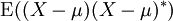
10. Computational formula for variance
The computational formula for the variance follows in a straightforward manner from the linearity of expected values and the above definition:


 This is often used to calculate the variance in practice, although it suffers from
numerical approximation
error
if the two components of the equation are similar in magnitude.
This is often used to calculate the variance in practice, although it suffers from
numerical approximation
error
if the two components of the equation are similar in magnitude.Characteristic propertyThe second moment of a random variable attains the minimum value when taken around the mean of the random variable, i.e. EX = argminaE(X − a)2. This property could be reversed, i.e. if the function φ satisfies EX = argminaEφ(X − a) then it is necessary of the form φ = ax2 + b. This is also true in multidimensional case [1] .
Approximating the variance of a functionThe delta method uses second-order Taylor expansions to approximate the variance of a function of one or more randomvariables. For example, the approximate variance of a function of onevariable is given by
 provided that f is twice differentiable and that the mean and variance of X are finite.
Population variance and sample varianceIn general, the population variance of a finite population of size N is given by
 or if the population is an
abstract population
with probability distribution Pr:
or if the population is an
abstract population
with probability distribution Pr: where
where
 is the population mean. This is merely a special case of the generaldefinition of variance introduced above, but restricted to finitepopulations.
In many practical situations, the true variance of a population is not known a priori and must be computed somehow. When dealing with infinite populations, this is generally impossible.
A common method is estimating the variance of large (finite or infinite) populations from a sample . We take a sample
 of nvalues from the population, and estimate the variance on the basis ofthis sample. There are several good estimators. Two of them are wellknown:
 and
and Both are referred to as
sample variance
. Most advanced electronic calculators can calculate both
Both are referred to as
sample variance
. Most advanced electronic calculators can calculate both
 and s2at the press of a button, in which case that button is usually labeled σ2 or
 for
and
for
and
 for s2.
The two estimators only differ slightly as we see, and for larger values of the sample size n the difference is negligible. The second one is an unbiased estimator of the population variance, meaning that its expected value E[s2]is equal to the true variance of the sampled random variable. The firstone may be seen as the variance of the sample considered as apopulation.
Common sense would suggest to apply the population formula to thesample as well. The reason that it is biased is that the sample mean isgenerally somewhat closer to the observations in the sample than thepopulation mean is to these observations. This is so because the samplemean is by definition in the middle of the sample, while the populationmean may even lie outside the sample. So the deviations to the samplemean will often be smaller than the deviations to the population mean,and so, if the same formula is applied to both, then this varianceestimate will on average be somewhat smaller in the sample than in thepopulation.
One common source of confusion is that the term sample variance may refer to either the unbiased estimator s2 of the population variance, or to the variance σ2of the sample viewed as a finite population. Both can be used toestimate the true population variance. Apart from theoreticalconsiderations, it doesn't really matter which one is used, as forsmall sample sizes both are inaccurate and for large values of n they are practically the same. Naively computing the variance by dividing by n instead of n-1systematically underestimates the population variance. Moreover, inpractical applications most people report the standard deviation ratherthan the sample variance, and the standard deviation that is obtainedfrom the unbiased n-1 version of the sample variance has aslight negative bias (though for normally distributed samples atheoretically interesting but rarely used slight correction exists to eliminate this bias). Nevertheless, in applied statistics it is a convention to use the n-1 version if the variance or the standard deviation is computed from a sample.
In practice, for large n, thedistinction is often a minor one. In the course of statisticalmeasurements, sample sizes so small as to warrant the use of theunbiased variance virtually never occur. In this context Press et al. [2] commented that if the difference between n and n−1ever matters to you, then you are probably up to no good anyway - e.g.,trying to substantiate a questionable hypothesis with marginal data.
Distribution of the sample varianceBeing a function of random variables , the sample variance is itself a random variable, and it is natural to study its distribution. In the case that yi are independent observations from a normal distribution , Cochran's theorem shows that s2 follows a scaled chi-square distribution :
 As a direct consequence, it follows that
 .
.However, even in the absence of the Normal assumption, it is still possible to prove that s2 is unbiased for σ2.
GeneralizationsIf X is a vector -valued random variable, with values in
 , and thought of as a column vector, then the natural generalization of variance is
 , where
 and
and
 is the transpose of X, and so is a row vector. This variance is a
positive semi-definite square matrix
, commonly referred to as the
covariance matrix
.
is the transpose of X, and so is a row vector. This variance is a
positive semi-definite square matrix
, commonly referred to as the
covariance matrix
.If X is a complex -valued random variable, with values in
 , then its variance is
 , where X * is the
complex conjugate
of X. This variance is also a positive semi-definite square matrix.
, where X * is the
complex conjugate
of X. This variance is also a positive semi-definite square matrix.HistoryThe term variance was first introduced by Ronald Fisher in his 1918 paper The Correlation Between Relatives on the Supposition of Mendelian Inheritance [3] :
[indent]The great body of available statistics show us that the deviations of a human measurement from its mean follow very closely the Normal Law of Errors , and, therefore, that the variability may be uniformly measured by the standard deviation corresponding to the square root of the mean square error .When there are two independent causes of variability capable ofproducing in an otherwise uniform population distributions withstandard deviations θ1 and θ2, it is found that the distribution, when both causes act together, has a standard deviation
 .It is therefore desirable in analysing the causes of variability todeal with the square of the standard deviation as the measure ofvariability. We shall term this quantity the Variance...
[/indent]
Moment of inertiaThe variance of a probability distribution is analogous to the moment of inertia in classical mechanics of a corresponding mass distribution along a line, with respect torotation about its center of mass. It is because of this analogy thatsuch things as the variance are called moments of probability distributions . (The covariance matrix is analogous to the moment of inertia tensor for multivariate distributions.)
Related Topics:
See Definition of Beta
